coursework
a project with a background image and giscus comments
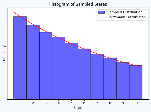
Exercise 1.1.
import numpy as np
import matplotlib.pyplot as plt
import random

# Boltzmann distribution for x states

def boltzmann_factor(beta: np.ndarray) -> np.ndarray:
    boltzmann = np.exp(-beta)
    Z = np.sum(boltzmann)
    return boltzmann / Z


# Define the states and their probabilities

x = np.arange(1, 11, 1)
beta = 0.1 * x
boltzmann_probs = boltzmann_factor(beta)
n = 100000


# Sample from the Boltzmann distribution

def sample_boltzmann(boltzmann_probs):
    u = random.uniform(0, 1)
    P = boltzmann_probs[0]
    i = 0
    while u >= P:
        i += 1
        P += boltzmann_probs[i]
    return x[i]

# Sample
samples = np.zeros(n, dtype=int)
for k in range(n):
    sample = sample_boltzmann(boltzmann_probs)
    samples[k] = sample


# background color as \definecolor{figurebg}{RGB}{245, 248, 252}
# Plot histogram
plt.figure(facecolor='#F5F8FC')
plt.hist(samples, bins=np.arange(1, 12)-0.5, density=True, alpha=0.6, color='b', label='Sampled Distribution', edgecolor = 'black')
x = np.linspace(0.5, 10.5, 100)
plt.plot(x, boltzmann_factor(0.1 * x)*10, 'r-', label='Boltzmann Distribution') # Factor 10 to counter the normalization constant (pΔx)
plt.xlabel('State')
plt.xticks(np.arange(1, 11, 1))
plt.yticks([])
plt.ylabel('Probability')
plt.title('Histogram of Sampled States')
plt.legend()
plt.tight_layout()
plt.savefig('H1-LaTeX/img/exercise_1_1_histogram.pdf', dpi=300)
plt.show()
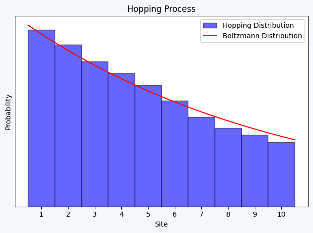
Exercise 1.2.
# Define hopping matrix

def hopping_matrix(s, t):
    """
        s: current state
        t: next state
    """
    if s == 0:
        if t == 0:
            return 1 - 0.5 * np.exp(-0.1)
        elif t == 1:
            return 0.5 * np.exp(-0.1)
        else:
            return 0

    if s == 9:
        if t == 8:
            return 0.5
        elif t == 9:
            return 0.5
        else:
            return 0

    if t == s - 1:
        return 0.5
    if t == s + 1:
        return 0.5 * np.exp(-0.1)
    if t == s:
        return 0.5 * (1 - np.exp(-0.1))
    return 0

# Calculate the hopping matrix once - saved just 0.1s of 1.4s :/ -> defining and sites = np.zeros(n+1, dtype=int) instead of appending to a list saved a lot!!


H = np.zeros((10, 10))

for s in range(10):
    for t in range(10):
        H[s, t] = hopping_matrix(s, t) # s is current state, t is next state

# starting point x0:

x0 = 0

n = 100000
sites = np.zeros(n+1, dtype=int)
sites[0] = x0


for k in range(n):
    current_site = sites[k]
    u = random.uniform(0, 1)
    next_site = 0
    P = H[current_site, next_site]
    while u > P:
        next_site += 1
        P += H[current_site, next_site]
    sites[k+1] = next_site


plt.figure(facecolor='#F5F8FC')
plt.hist(sites+1, bins=np.arange(0.5, 11.5, 1), density=True, edgecolor = 'black', alpha=0.6, color='b', label='Hopping Distribution')
x = np.linspace(0.5, 10.5, 100)
plt.plot(x, boltzmann_factor(0.1 * x)*10, 'r-', label='Boltzmann Distribution') # Factor 10 to counter the normalization constant (pΔx)
plt.xlabel("Site")
plt.yticks([])
plt.xticks(np.arange(1, 11, 1))
plt.ylabel("Probability")
plt.title("Hopping Process")
plt.legend()
plt.tight_layout()
plt.savefig('H1-LaTeX/img/exercise_1_2_histogram.pdf', dpi=300)
plt.show()
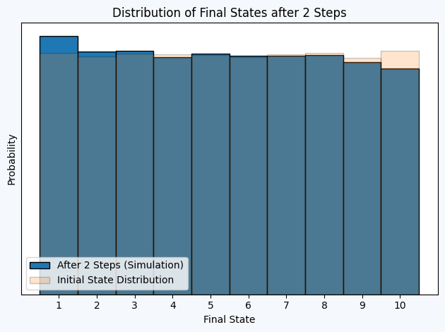
Exercise 1.3.
# doing multiple processes with 2 steps!
n = 100000
samples = np.zeros((3, n), dtype=int) # initial states, at start, after 1 step, after 2 steps
def one_step(site):
u = random.uniform(0, 1)
for k in range(10):
P = H[site, 0]
k = 0
while u >= P:
k += 1
P += H[site, k]
return k
for i in range(n):
samples[0, i] = random.randint(0, 9)
samples[1, i] = one_step(samples[0, i])
samples[2, i] = one_step(samples[1, i])
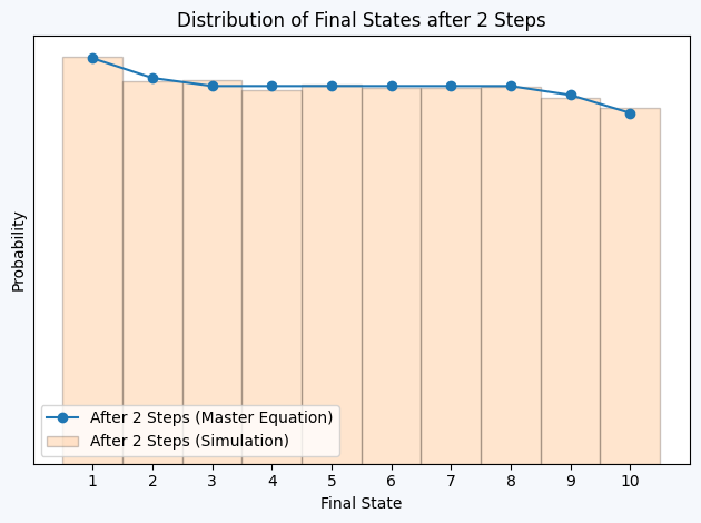
plt.figure(facecolor='#F5F8FC')
plt.hist(samples[2, :]+1, bins=np.arange(0.5, 11.5, 1), density=True, label='After 2 Steps (Simulation)', edgecolor = 'black')
plt.hist(samples[0, :]+1, bins=np.arange(0.5, 11.5, 1), density=True, alpha=0.2, edgecolor = 'black', label='Initial State Distribution')
plt.xlabel("Final State")
plt.xticks(np.arange(1, 11, 1))
plt.yticks([])
plt.ylabel("Probability")
plt.title("Distribution of Final States after 2 Steps")
plt.legend(loc='lower left')
plt.tight_layout()
plt.savefig('H1-LaTeX/img/exercise_1_3_MChistogram.pdf', dpi=300)
plt.show()
# Using Master equation!
P = np.ones(10) / 10 # Initial uniform distribution
P1 = np.zeros(10)
for k in range(10):
for i in range(10):
P1[i] += H[k, i] * P[k]
P2 = np.zeros(10)
for k in range(10):
for i in range(10):
P2[i] += H[k, i] * P1[k]
plt.figure(facecolor='#F5F8FC')
plt.plot(np.arange(1, 11), P2, label='After 2 Steps (Master Equation)', marker='o')
plt.hist(samples[2, :]+1, bins=np.arange(0.5, 11.5, 1), density=True, alpha=0.2, edgecolor = 'black', label='After 2 Steps (Simulation)')
plt.xlabel("Final State")
plt.xticks(np.arange(1, 11, 1))
plt.yticks([])
plt.ylabel("Probability")
plt.title("Distribution of Final States after 2 Steps")
plt.legend()
plt.tight_layout()
plt.savefig('H1-LaTeX/img/exercise_1_3_MEmatch.pdf', dpi=300)
plt.show()
Exercise 1.4.
\(P^*_x = \frac{1}{Z} \exp(-\beta E_x)\) with \(\beta E_x = 0.1 x\) Assuming only nearest neighbor interactions \(\frac{1}{2}\cdot\begin{pmatrix} 0 & 1 & 0 & 0 & 0 \\ 1 & 0 & 1 & 0 & 0 \\ 0 & 1 & 0 & 1 & 0 \\ 0 & 0 & 1 & 0 & 1 \\ 0 & 0 & 0 & 1 & 0 \end{pmatrix}\)
Exercise 1.5.
some analytical stuffff
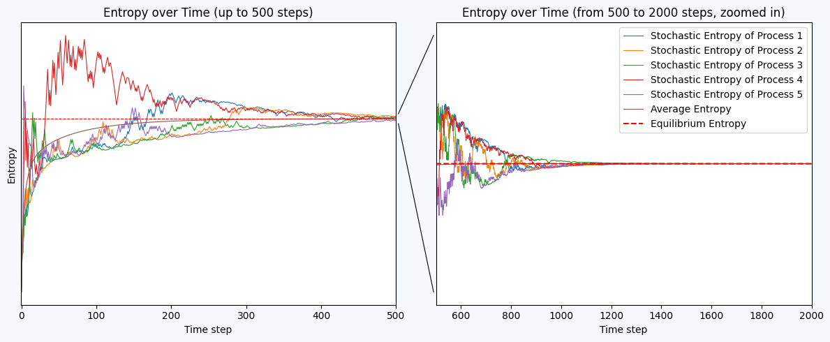
Exercise 1.6.
discrete gaussian
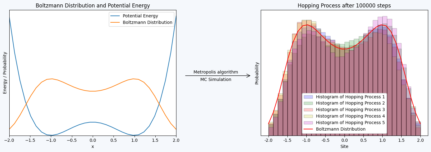
Potential: \(V(x) = x^4 - 2x^2 + 1\)
32 states from $x=-2$ to $x=2$
def potential (x):
    return x**4 - 2 * x**2 + 1

def monte_carlo(x0, n, k):
    """
        x0: starting point
        n: number of steps
        k: transition matrix
    """
    sites = np.zeros(n+1, dtype=int)
    sites[0] = x0
    for l in range(n):
        current_site = sites[l]
        u = random.uniform(0, 1)
        next_site = 0
        P = k[next_site, current_site]
        while u >= P:
            next_site += 1
            P += k[next_site, current_site]

        sites[l+1] = next_site
    return sites

# define my states in space
ε = 32
n = 100000
beta = 0.25


x = np.linspace(-2, 2, ε)

E_x = potential(x)
P_x = np.exp(-beta * E_x)
P_x /= np.sum(P_x)


# Q for nearest neighbor jumps only
Q = np.zeros((ε,ε))
for i in range(ε-1):
    Q[i,i+1] = 0.5
    Q[i+1,i] = 0.5

# now caluclate A

A = np.zeros((ε,ε))
for i in range(ε-1):
    A[i,i+1] = min(1, P_x[i]/P_x[i+1])
    A[i+1,i] = min(1, P_x[i+1]/P_x[i])

k = A * Q

for i in range(ε):
    k[i,i] = 1 - np.sum(k[:,i])

# print k as LaTeX matrix
# sp?
import sympy as sp
k_matrix = sp.Matrix(np.round(k, 2))
k_latex = sp.latex(k_matrix)
print(k_latex)

# starting point x0:

x0 = random.randint(0, ε-1)

# run the Monte Carlo simulation
sites = monte_carlo(x0, n, k)
sites1 = monte_carlo(x0, n, k)
sites2 = monte_carlo(x0, n, k)
sites3 = monte_carlo(x0, n, k)
sites4 = monte_carlo(x0, n, k)
\left[\begin{array}{cccccccccccccccccccccccccccccccc}0.5 & 0.25 & 0.0 & 0.0 & 0.0 & 0.0 & 0.0 & 0.0 & 0.0 & 0.0 & 0.0 & 0.0 & 0.0 & 0.0 & 0.0 & 0.0 & 0.0 & 0.0 & 0.0 & 0.0 & 0.0 & 0.0 & 0.0 & 0.0 & 0.0 & 0.0 & 0.0 & 0.0 & 0.0 & 0.0 & 0.0 & 0.0\\0.5 & 0.25 & 0.29 & 0.0 & 0.0 & 0.0 & 0.0 & 0.0 & 0.0 & 0.0 & 0.0 & 0.0 & 0.0 & 0.0 & 0.0 & 0.0 & 0.0 & 0.0 & 0.0 & 0.0 & 0.0 & 0.0 & 0.0 & 0.0 & 0.0 & 0.0 & 0.0 & 0.0 & 0.0 & 0.0 & 0.0 & 0.0\\0.0 & 0.5 & 0.21 & 0.34 & 0.0 & 0.0 & 0.0 & 0.0 & 0.0 & 0.0 & 0.0 & 0.0 & 0.0 & 0.0 & 0.0 & 0.0 & 0.0 & 0.0 & 0.0 & 0.0 & 0.0 & 0.0 & 0.0 & 0.0 & 0.0 & 0.0 & 0.0 & 0.0 & 0.0 & 0.0 & 0.0 & 0.0\\0.0 & 0.0 & 0.5 & 0.16 & 0.38 & 0.0 & 0.0 & 0.0 & 0.0 & 0.0 & 0.0 & 0.0 & 0.0 & 0.0 & 0.0 & 0.0 & 0.0 & 0.0 & 0.0 & 0.0 & 0.0 & 0.0 & 0.0 & 0.0 & 0.0 & 0.0 & 0.0 & 0.0 & 0.0 & 0.0 & 0.0 & 0.0\\0.0 & 0.0 & 0.0 & 0.5 & 0.12 & 0.41 & 0.0 & 0.0 & 0.0 & 0.0 & 0.0 & 0.0 & 0.0 & 0.0 & 0.0 & 0.0 & 0.0 & 0.0 & 0.0 & 0.0 & 0.0 & 0.0 & 0.0 & 0.0 & 0.0 & 0.0 & 0.0 & 0.0 & 0.0 & 0.0 & 0.0 & 0.0\\0.0 & 0.0 & 0.0 & 0.0 & 0.5 & 0.09 & 0.45 & 0.0 & 0.0 & 0.0 & 0.0 & 0.0 & 0.0 & 0.0 & 0.0 & 0.0 & 0.0 & 0.0 & 0.0 & 0.0 & 0.0 & 0.0 & 0.0 & 0.0 & 0.0 & 0.0 & 0.0 & 0.0 & 0.0 & 0.0 & 0.0 & 0.0\\0.0 & 0.0 & 0.0 & 0.0 & 0.0 & 0.5 & 0.05 & 0.47 & 0.0 & 0.0 & 0.0 & 0.0 & 0.0 & 0.0 & 0.0 & 0.0 & 0.0 & 0.0 & 0.0 & 0.0 & 0.0 & 0.0 & 0.0 & 0.0 & 0.0 & 0.0 & 0.0 & 0.0 & 0.0 & 0.0 & 0.0 & 0.0\\0.0 & 0.0 & 0.0 & 0.0 & 0.0 & 0.0 & 0.5 & 0.03 & 0.5 & 0.0 & 0.0 & 0.0 & 0.0 & 0.0 & 0.0 & 0.0 & 0.0 & 0.0 & 0.0 & 0.0 & 0.0 & 0.0 & 0.0 & 0.0 & 0.0 & 0.0 & 0.0 & 0.0 & 0.0 & 0.0 & 0.0 & 0.0\\0.0 & 0.0 & 0.0 & 0.0 & 0.0 & 0.0 & 0.0 & 0.5 & 0.02 & 0.5 & 0.0 & 0.0 & 0.0 & 0.0 & 0.0 & 0.0 & 0.0 & 0.0 & 0.0 & 0.0 & 0.0 & 0.0 & 0.0 & 0.0 & 0.0 & 0.0 & 0.0 & 0.0 & 0.0 & 0.0 & 0.0 & 0.0\\0.0 & 0.0 & 0.0 & 0.0 & 0.0 & 0.0 & 0.0 & 0.0 & 0.49 & 0.02 & 0.5 & 0.0 & 0.0 & 0.0 & 0.0 & 0.0 & 0.0 & 0.0 & 0.0 & 0.0 & 0.0 & 0.0 & 0.0 & 0.0 & 0.0 & 0.0 & 0.0 & 0.0 & 0.0 & 0.0 & 0.0 & 0.0\\0.0 & 0.0 & 0.0 & 0.0 & 0.0 & 0.0 & 0.0 & 0.0 & 0.0 & 0.48 & 0.02 & 0.5 & 0.0 & 0.0 & 0.0 & 0.0 & 0.0 & 0.0 & 0.0 & 0.0 & 0.0 & 0.0 & 0.0 & 0.0 & 0.0 & 0.0 & 0.0 & 0.0 & 0.0 & 0.0 & 0.0 & 0.0\\0.0 & 0.0 & 0.0 & 0.0 & 0.0 & 0.0 & 0.0 & 0.0 & 0.0 & 0.0 & 0.48 & 0.02 & 0.5 & 0.0 & 0.0 & 0.0 & 0.0 & 0.0 & 0.0 & 0.0 & 0.0 & 0.0 & 0.0 & 0.0 & 0.0 & 0.0 & 0.0 & 0.0 & 0.0 & 0.0 & 0.0 & 0.0\\0.0 & 0.0 & 0.0 & 0.0 & 0.0 & 0.0 & 0.0 & 0.0 & 0.0 & 0.0 & 0.0 & 0.48 & 0.02 & 0.5 & 0.0 & 0.0 & 0.0 & 0.0 & 0.0 & 0.0 & 0.0 & 0.0 & 0.0 & 0.0 & 0.0 & 0.0 & 0.0 & 0.0 & 0.0 & 0.0 & 0.0 & 0.0\\0.0 & 0.0 & 0.0 & 0.0 & 0.0 & 0.0 & 0.0 & 0.0 & 0.0 & 0.0 & 0.0 & 0.0 & 0.48 & 0.02 & 0.5 & 0.0 & 0.0 & 0.0 & 0.0 & 0.0 & 0.0 & 0.0 & 0.0 & 0.0 & 0.0 & 0.0 & 0.0 & 0.0 & 0.0 & 0.0 & 0.0 & 0.0\\0.0 & 0.0 & 0.0 & 0.0 & 0.0 & 0.0 & 0.0 & 0.0 & 0.0 & 0.0 & 0.0 & 0.0 & 0.0 & 0.48 & 0.01 & 0.5 & 0.0 & 0.0 & 0.0 & 0.0 & 0.0 & 0.0 & 0.0 & 0.0 & 0.0 & 0.0 & 0.0 & 0.0 & 0.0 & 0.0 & 0.0 & 0.0\\0.0 & 0.0 & 0.0 & 0.0 & 0.0 & 0.0 & 0.0 & 0.0 & 0.0 & 0.0 & 0.0 & 0.0 & 0.0 & 0.0 & 0.49 & 0.0 & 0.5 & 0.0 & 0.0 & 0.0 & 0.0 & 0.0 & 0.0 & 0.0 & 0.0 & 0.0 & 0.0 & 0.0 & 0.0 & 0.0 & 0.0 & 0.0\\0.0 & 0.0 & 0.0 & 0.0 & 0.0 & 0.0 & 0.0 & 0.0 & 0.0 & 0.0 & 0.0 & 0.0 & 0.0 & 0.0 & 0.0 & 0.5 & 0.0 & 0.49 & 0.0 & 0.0 & 0.0 & 0.0 & 0.0 & 0.0 & 0.0 & 0.0 & 0.0 & 0.0 & 0.0 & 0.0 & 0.0 & 0.0\\0.0 & 0.0 & 0.0 & 0.0 & 0.0 & 0.0 & 0.0 & 0.0 & 0.0 & 0.0 & 0.0 & 0.0 & 0.0 & 0.0 & 0.0 & 0.0 & 0.5 & 0.01 & 0.48 & 0.0 & 0.0 & 0.0 & 0.0 & 0.0 & 0.0 & 0.0 & 0.0 & 0.0 & 0.0 & 0.0 & 0.0 & 0.0\\0.0 & 0.0 & 0.0 & 0.0 & 0.0 & 0.0 & 0.0 & 0.0 & 0.0 & 0.0 & 0.0 & 0.0 & 0.0 & 0.0 & 0.0 & 0.0 & 0.0 & 0.5 & 0.02 & 0.48 & 0.0 & 0.0 & 0.0 & 0.0 & 0.0 & 0.0 & 0.0 & 0.0 & 0.0 & 0.0 & 0.0 & 0.0\\0.0 & 0.0 & 0.0 & 0.0 & 0.0 & 0.0 & 0.0 & 0.0 & 0.0 & 0.0 & 0.0 & 0.0 & 0.0 & 0.0 & 0.0 & 0.0 & 0.0 & 0.0 & 0.5 & 0.02 & 0.48 & 0.0 & 0.0 & 0.0 & 0.0 & 0.0 & 0.0 & 0.0 & 0.0 & 0.0 & 0.0 & 0.0\\0.0 & 0.0 & 0.0 & 0.0 & 0.0 & 0.0 & 0.0 & 0.0 & 0.0 & 0.0 & 0.0 & 0.0 & 0.0 & 0.0 & 0.0 & 0.0 & 0.0 & 0.0 & 0.0 & 0.5 & 0.02 & 0.48 & 0.0 & 0.0 & 0.0 & 0.0 & 0.0 & 0.0 & 0.0 & 0.0 & 0.0 & 0.0\\0.0 & 0.0 & 0.0 & 0.0 & 0.0 & 0.0 & 0.0 & 0.0 & 0.0 & 0.0 & 0.0 & 0.0 & 0.0 & 0.0 & 0.0 & 0.0 & 0.0 & 0.0 & 0.0 & 0.0 & 0.5 & 0.02 & 0.48 & 0.0 & 0.0 & 0.0 & 0.0 & 0.0 & 0.0 & 0.0 & 0.0 & 0.0\\0.0 & 0.0 & 0.0 & 0.0 & 0.0 & 0.0 & 0.0 & 0.0 & 0.0 & 0.0 & 0.0 & 0.0 & 0.0 & 0.0 & 0.0 & 0.0 & 0.0 & 0.0 & 0.0 & 0.0 & 0.0 & 0.5 & 0.02 & 0.49 & 0.0 & 0.0 & 0.0 & 0.0 & 0.0 & 0.0 & 0.0 & 0.0\\0.0 & 0.0 & 0.0 & 0.0 & 0.0 & 0.0 & 0.0 & 0.0 & 0.0 & 0.0 & 0.0 & 0.0 & 0.0 & 0.0 & 0.0 & 0.0 & 0.0 & 0.0 & 0.0 & 0.0 & 0.0 & 0.0 & 0.5 & 0.02 & 0.5 & 0.0 & 0.0 & 0.0 & 0.0 & 0.0 & 0.0 & 0.0\\0.0 & 0.0 & 0.0 & 0.0 & 0.0 & 0.0 & 0.0 & 0.0 & 0.0 & 0.0 & 0.0 & 0.0 & 0.0 & 0.0 & 0.0 & 0.0 & 0.0 & 0.0 & 0.0 & 0.0 & 0.0 & 0.0 & 0.0 & 0.5 & 0.03 & 0.5 & 0.0 & 0.0 & 0.0 & 0.0 & 0.0 & 0.0\\0.0 & 0.0 & 0.0 & 0.0 & 0.0 & 0.0 & 0.0 & 0.0 & 0.0 & 0.0 & 0.0 & 0.0 & 0.0 & 0.0 & 0.0 & 0.0 & 0.0 & 0.0 & 0.0 & 0.0 & 0.0 & 0.0 & 0.0 & 0.0 & 0.47 & 0.05 & 0.5 & 0.0 & 0.0 & 0.0 & 0.0 & 0.0\\0.0 & 0.0 & 0.0 & 0.0 & 0.0 & 0.0 & 0.0 & 0.0 & 0.0 & 0.0 & 0.0 & 0.0 & 0.0 & 0.0 & 0.0 & 0.0 & 0.0 & 0.0 & 0.0 & 0.0 & 0.0 & 0.0 & 0.0 & 0.0 & 0.0 & 0.45 & 0.09 & 0.5 & 0.0 & 0.0 & 0.0 & 0.0\\0.0 & 0.0 & 0.0 & 0.0 & 0.0 & 0.0 & 0.0 & 0.0 & 0.0 & 0.0 & 0.0 & 0.0 & 0.0 & 0.0 & 0.0 & 0.0 & 0.0 & 0.0 & 0.0 & 0.0 & 0.0 & 0.0 & 0.0 & 0.0 & 0.0 & 0.0 & 0.41 & 0.12 & 0.5 & 0.0 & 0.0 & 0.0\\0.0 & 0.0 & 0.0 & 0.0 & 0.0 & 0.0 & 0.0 & 0.0 & 0.0 & 0.0 & 0.0 & 0.0 & 0.0 & 0.0 & 0.0 & 0.0 & 0.0 & 0.0 & 0.0 & 0.0 & 0.0 & 0.0 & 0.0 & 0.0 & 0.0 & 0.0 & 0.0 & 0.38 & 0.16 & 0.5 & 0.0 & 0.0\\0.0 & 0.0 & 0.0 & 0.0 & 0.0 & 0.0 & 0.0 & 0.0 & 0.0 & 0.0 & 0.0 & 0.0 & 0.0 & 0.0 & 0.0 & 0.0 & 0.0 & 0.0 & 0.0 & 0.0 & 0.0 & 0.0 & 0.0 & 0.0 & 0.0 & 0.0 & 0.0 & 0.0 & 0.34 & 0.21 & 0.5 & 0.0\\0.0 & 0.0 & 0.0 & 0.0 & 0.0 & 0.0 & 0.0 & 0.0 & 0.0 & 0.0 & 0.0 & 0.0 & 0.0 & 0.0 & 0.0 & 0.0 & 0.0 & 0.0 & 0.0 & 0.0 & 0.0 & 0.0 & 0.0 & 0.0 & 0.0 & 0.0 & 0.0 & 0.0 & 0.0 & 0.29 & 0.25 & 0.5\\0.0 & 0.0 & 0.0 & 0.0 & 0.0 & 0.0 & 0.0 & 0.0 & 0.0 & 0.0 & 0.0 & 0.0 & 0.0 & 0.0 & 0.0 & 0.0 & 0.0 & 0.0 & 0.0 & 0.0 & 0.0 & 0.0 & 0.0 & 0.0 & 0.0 & 0.0 & 0.0 & 0.0 & 0.0 & 0.0 & 0.25 & 0.5\end{array}\right]
Plots separately
fig, ax = plt.subplots(1, 2, figsize=(14,5), facecolor='#F5F8FC')
# First subplot
ax[0].plot(x, potential(x),  label='Potential Energy')
ax[0].plot(x, P_x*100,  label='Boltzmann Distribution') # Factor 10 to counter the normalization constant (pΔx)
ax[0].set_title("Boltzmann Distribution and Potential Energy")
ax[0].set_xlabel("x")
ax[0].set_ylabel("Energy / Probability")
ax[0].set_yticks([])


from matplotlib.patches import FancyArrowPatch

arrow = FancyArrowPatch((2.2, 4.5), (3.8, 4.5),  # von Punkt A zu Punkt B
                       arrowstyle='->', mutation_scale=20,
                       color='black', linewidth=1, clip_on=False)
ax[0].add_patch(arrow)
ax[0].text(2.95, 4.6, 'Metropolis algorithm', fontsize=10, ha='center', va='bottom')
ax[0].text(2.95, 4.35, 'MC Simulation', fontsize=10, ha='center', va='top')
# just a gap!
ax[0].text(3.9, 4.5, 'P', fontsize=10, ha='center', va='center', color='#F5F8FC')


ax[0].set_xlim(-2,2)
# just lower bound for y-axis
ax[0].set_ylim(bottom = -0.01)
ax[0].legend()


# Second subplot
ax[1].hist(sites+1, bins=np.arange(1, 34, 1), density=True, edgecolor = 'black', alpha=0.2, color='b', label='Histogram of Hopping Process 1')
ax[1].hist(sites1+1, bins=np.arange(1, 34, 1), density=True, edgecolor = 'black', alpha=0.2, color='g', label='Histogram of Hopping Process 2')
ax[1].hist(sites2+1, bins=np.arange(1, 34, 1), density=True, edgecolor = 'black', alpha=0.2, color='r', label='Histogram of Hopping Process 3')
ax[1].hist(sites3+1, bins=np.arange(1, 34, 1), density=True, edgecolor = 'black', alpha=0.2, color='y', label='Histogram of Hopping Process 4')
ax[1].hist(sites4+1, bins=np.arange(1, 34, 1), density=True, edgecolor = 'black', alpha=0.2, color='m', label='Histogram of Hopping Process 5')
ax[1].plot((x+2)*32/4+1, P_x, 'r-', label='Boltzmann Distribution') # Factor 10 to counter the normalization constant (pΔx)
ax[1].set_xlabel("Site")
#ax[1].set_ylabel("Probability")


ax[1].set_ylabel("Probability")
ax[1].set_yticks([])
ax[1].set_xticks(np.arange(1, 34, 4))
ax[1].set_xticklabels(np.round(np.arange(-2, 2.1, 4/8), 2))
ax[1].set_title("Hopping Process after "+str(n)+" steps")
ax[1].legend(loc='lower center', framealpha=1)

plt.tight_layout()
#plt.savefig('H1-LaTeX/img/exercise_1_6_histogram.pdf', dpi=300)
plt.show()
P_stoch = np.zeros((ε, n+1))
P_stoch[sites[0], 0] = 1

for t in range(n):
    P_stoch[:, t+1] = k @ P_stoch[:, t]


def entropy(sites, P_stoch, P_eq, t):
    return - np.log(P_stoch[sites[t], t] / P_eq[sites[t]])

def summ(P_stoch, P_eq, ε, t):
    S = 0
    for i in range(ε):
        if P_stoch[i, t] == 0:
            continue
        S += - P_stoch[i, t] * np.log(P_stoch[i, t] / P_eq[i])
    return S

n = 2000
time = np.arange(n+1)

S = np.zeros(n+1)
S1 = np.zeros(n+1)
S2 = np.zeros(n+1)
S3 = np.zeros(n+1)
S4 = np.zeros(n+1)
S_tot = np.zeros(n+1)
for t in time:
    S[t] = entropy(sites, P_stoch, P_x, t)
    S1[t] = entropy(sites1, P_stoch, P_x, t)
    S2[t] = entropy(sites2, P_stoch, P_x, t)
    S3[t] = entropy(sites3, P_stoch, P_x, t)
    S4[t] = entropy(sites4, P_stoch, P_x, t)
    S_tot[t] = summ(P_stoch, P_x, ε, t)


# Join last two plots in one subfigure (deleted the last two plots and made a subplot instead)

fig, ax = plt.subplots(1, 2, figsize=(12, 5), facecolor='#F5F8FC')
# First subplot
ax[0].plot(time, S, linewidth=0.8)
ax[0].plot(time, S1, linewidth=0.8)
ax[0].plot(time, S2, linewidth=0.8)
ax[0].plot(time, S3, linewidth=0.8)
ax[0].plot(time, S4, linewidth=0.8)
ax[0].plot(time, S_tot, linewidth=0.8)
ax[0].plot(time, 0*S, 'r--', linewidth=0.8)
# Zoom like effect!

x = np.array([503, 550])
y = np.array([-0.09, min(S)])

ax[0].plot(x, y, 'k-', clip_on=False, scalex=False, scaley=False, linewidth=0.8)

x = np.array([503, 550])
y = np.array([0.09, max([max(S), max(S1), max(S2), max(S3), max(S4), max(S_tot)])])

ax[0].plot(x, y, 'k-', clip_on=False, scalex=False, scaley=False, linewidth=0.8)

ax[0].set_xlabel("Time step")
ax[0].set_ylabel("Entropy")
ax[0].set_yticks([])
ax[0].set_title("Entropy over Time (up to 500 steps)")
#ax[0].legend()
ax[0].set_xlim(-1, 500)
# Second subplot
ax[1].plot(time, S, label='Stochastic Entropy of Process 1', linewidth=0.8)
ax[1].plot(time, S1, label='Stochastic Entropy of Process 2', linewidth=0.8)
ax[1].plot(time, S2, label='Stochastic Entropy of Process 3', linewidth=0.8)
ax[1].plot(time, S3, label='Stochastic Entropy of Process 4', linewidth=0.8)
ax[1].plot(time, S4, label='Stochastic Entropy of Process 5', linewidth=0.8)
ax[1].plot(time, S_tot, label='Average Entropy', linewidth=0.8)
ax[1].plot(time, 0*S, 'r--', label='Equilibrium Entropy')
ax[1].set_xlabel("Time step")
#ax[1].set_ylabel("Entropy")
ax[1].set_yticks([])
ax[1].set_title("Entropy over Time (from 500 to 2000 steps, zoomed in)")
ax[1].legend()
ax[1].set_xlim(500, 2000)
ax[1].set_ylim(-0.1,0.1)
plt.tight_layout()
#plt.savefig('H1-LaTeX/img/exercise_1_6_entropy.pdf', dpi=300)
plt.show()